Region based classification fusion

The standard workflow use the region shape to crop each classification to avoid overlapping between regions. Once masked the classifications of each tiles are merged into one before generate the final complete mosaïc.

This handling can create artefacts in maps if the models are very different. Indeed, looking at a forest of pine which is covered by two regions, but one region did know the pine class, the pixels are then classified into another class. The following figure show the kind of issues which can occurs. The region boundary clearly appears in the produced map.

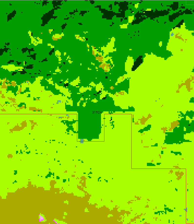
example of boundary artefact — Example of boundary artefact

A simple solution was proposed to smooth the boundary effect. Instead of applying a classification mask defined by the region vector, a per class probabilities fusion scheme was considered. The main idea is to compute a weighted fusion according to the distance of a pixel with relation to the region boundary.

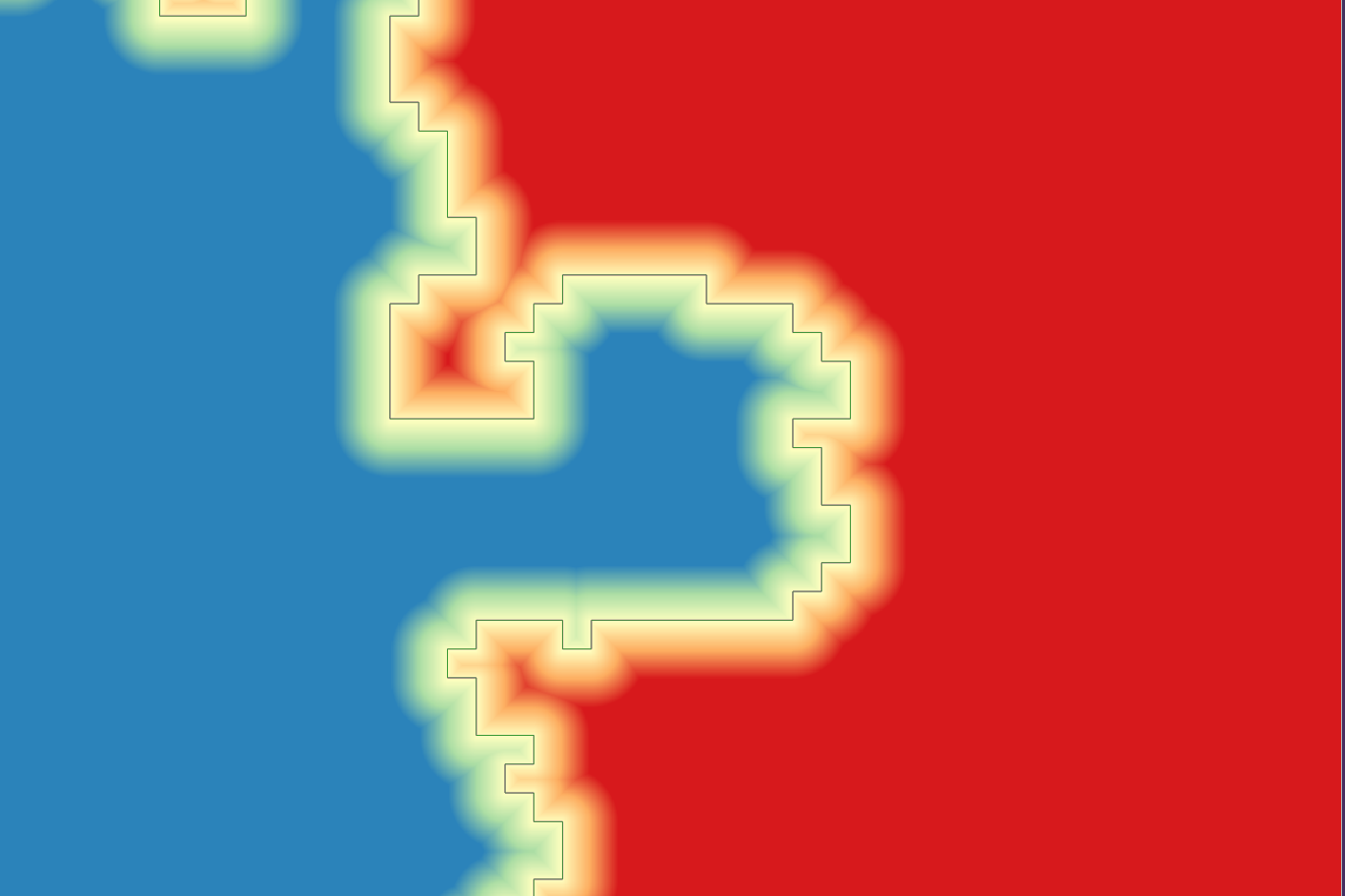
The definition of boundary is very important. As a vector shape file is considered to define regions and the maps is a raster, each pixel which intersect the boundary is defined as the region boundary in the map. According to this definition, it is possible to compute a buffer area around the boundary, and compute the distance of each pixel in this area with relation to the boundary. Then it is possible to define two new parameters: the interior_boundary and the exterior_boundary. The definition of interior and exterior is valid only for one region at the time. The buffer size to define interior and exterior boundary may be different. Considering a region, the interior buffer is defined as the area inside the region with relation to the original boundary.

The pixel’s distance to the boundary is computed using the Danielsson algorithm which compute euclidian distance in images.

The weight is computed with a linear expression, in order to provide a weight of 1 at the interior boundary, and a weight of 0 at the exterior boundary. A epsilon value is required to avoid O in weights if the region shape file geometry is complex. This value is a float which must be storable as UINT16 once multiplied by 1000, i.e the smallest values accepted is 0.001. Under this value, the weight is set to 0. At the original boundary, the weight is set to be 0.5.

Exemple of weights for the region 1 (red) and the region 2 (blue). The dark line is the boundary defined by the vector file. The weights compute are 0 outside the region (blue), 1 inside the region (red) and between 0 and 1 inside the buffer around the boundary.

After the classification of each region by a classifier which provides per class probability, a decision is taken by weighting the probability of each model by the pixel’s weight.

How to enable the boundary fusion mode

To enable the bonudary fusion, several parameters must be set.

Most of them are grouped in the arg_classification section of the configuration file.

arg_classification :
{
    enable_probability_map: True
    generate_final_probability_map: False
    boundary_comparison_mode:False
    enable_boundary_fusion: True
    boundary_interior_buffer_size: 100
    boundary_exterior_buffer_size: 500
    boundary_fusion_epsilon: 0.001
}

It is mandatory to enable the probability map production, as it is the main input of the workflow. The classifier set in the arg_train section must provide probabilities.

It is possible to set different value for the interior and exterior boundary size. Note that the unit is in meter here. The buffer size is converted in pixels according to the working resolution.

Use the comparison mode

It can be usefull to compare the two versions of merging classification.

To this end, an option was added boundary_comparison_mode. If enabled, the final folder is slighty modified to provided both version of all products: RESULTS.txt, Confusion matrix, land and confidence maps, in two separate subfolder: standard and boundary. At the root of final, some file are present containing conditional validation for the boundary areas only.

With the following convention:

\(C_s\) the fusion after masking the classification with regions

\(C_b\) the fusion using boundary area and probabilities

Four matrices and associated metrics are computed:

\(conf(C_s,Yref)\) : confusion matrix between \(C_s\) and the referenced points (not used during training) on the boundary

\(conf(C_b,Yref)\) : confusion matrix between \(C_b\) and the referenced points (not used during training) on the boundary

\(conf(C_s|Y=Yref, C_b)\) : confusion matrix between \(C_s\) only when the prediction of \(C_s\) are correct (correct = equal to the referenced points not used during training) and \(C_b\)

\(conf(C_b|Y=Yref, C_s)\) : confusion matrix between \(C_b\) only when the prediction of \(C_b\) are correct (correct = equal to the referenced points not used during training) and \(C_s\)