iota2 Training Labwork
Table of Contents
In the following, different extracts of the configuration file are provided. They do not correspond to a full configuration file, but it only shows where options need to be changed/set in the file to apply what it is discussed in the current section. Users should fill the remaining part by him/herself.
1. Practical Advice
1.1. Installation
For the labworks, an up to date iota\(^2\) conda package is required. Follow the documentation install procedure: https://docs.iota2.net/develop/HowToGetIOTA2.html
1.2. Data
Sample data can be found at https://docs.iota2.net/data/ in the i2_training_data.tar.bz2 archive which can be long to uncompress.
1.3. Labwork document
A html version of the labwork is available at https://docs.iota2.net/training/labworks.html
A pdf version of the labwork is available at https://docs.iota2.net/training/labworks.pdf
2. Training pixels sampling and model validation with iota2
This section deals with various advanced topics on time series classification with iota\(^2\). They were not covered during the introductory talk, but users need to understand them to correctly use iota\(^2\) for classification in real situation.
2.1. Training samples sampling parameters
The full documentation about pixels sampling can be found here: https://docs.iota2.net/develop/iota2_samples_management.html
As discussed in the general presentation, the initial ground truth data set is split into two spatially disjoints set, learn and val, provided splitGroundTruth is set to True. The split is done at the polygon level, i.e., one polygon from the ground-truth file will be assigned to either the learn or val set. The parameter ratio is used to control the number of polygons assigned to each set (the higher the ratio, the bigger the training set), on a class basis. It can be changed from the configuration file:
arg_train :
{
    ratio : 0.75  # 75% of the polygons are assigned to the learn dat set
    random_seed : 0 # Set the random seed to split the ground truth
}
Then, from the polygons in learn a subset of the available pixels are selected for training. For these operations, iota\(^2\) offers different strategies, based the OTB SampleSelection tool. It is possible to:
- Set the same number of extracted samples per class,
- Set the number extracted samples per class,
- Set the percentage of extracted samples per class,
- Set the total number of extracted samples, and use class pixels proportion to automatically set the number of extracted pixels per class,
- Use all the available samples.
Periodic or random selection are available when required. For instance, to select randomly 50% of the available pixels for each class the configuration file should be modified to:
arg_train :
{
    sampleSelection :
    {
        "sampler":"random",
        "strategy":"percent",
        "strategy.percent.p":0.5
        "rand" : 0 # In order to set the random seed for the sampleSelection app
    }
}
To change for a periodic sampling, just change to "sampler":"periodic". All the possible configurations are discussed in https://www.orfeo-toolbox.org/CookBook/Applications/app_SampleSelection.html and https://docs.iota2.net/develop/iota2_samples_management.html#sampleselection, along with more complex scenario (e.g. using regions).
Finally, whatever the sampling strategy, iota\(^2\) generates a report, called class_statistics.csv, with all the training samples per class, per region and per run (see next section for details about run).
The choice of the number of training and validation samples significantly influences the results of the classification. In this labwork, we ask you to test different strategies to sample training pixels. Using a fix ratio, try random and periodic selection with different strategy, i.e., a percentage of training pixels, a fix and common number of training pixels per class or a per-class number of pixels. For each configuration, take a look at the number of extracted samples.
All the required changes can be done in the configuration file.

If you asked for too many pixels in the training file, you might run into memory issues, since with conventional classifier, all the extracted pixels are load into memory for the learning step. Note that this issue is solved when using deep learning.
2.2. Multi-run
iota\(^2\) outputs the confusion matrix as well as some classification accuracy indices, for a given learning and test set (remind that randomness is controlled using the random seed parameters of iota\(^2\) and OTB, both adjustable from the configuration file). In order to better estimate those indices, several runs with random learning/testing set must be conducted.
iota\(^2\) offers the possibility to do it automatically by setting the parameter runs to a value higher than 1. For instance, to performs 10 classification, just change the configuration file to
arg_train :
{
    runs : 10
}
Number following the term seed in the files outputed by iota\(^2\) corresponds to the seed number, i.e., the run number: T31TCJ_seed_5_learn.sqlite is the training samples of the sixth runs. Consequently, with multiple runs, a lot of files are created.
With a reduce training sample to limit the computation burden, do several runs and look at the report file. Try to understand the meaning of its content. From all your configurations, which ones is the best in terms of classification accuracy ?
3. Advanced classification strategy
3.1. Deep Learning
Recently, iota\(^2\) has the ability to perform pixel-wise classification using deep neural network. In this section, we will show how to perform such classification. Most of the following is based on the documentation (https://docs.iota2.net/develop/deep_learning.html), we encourage users to read it deeply (!).
Currently, iota\(^2\) implement 4 algorithms: ‘LTAEClassifier’, ‘ANN’, ‘MLPClassifier’ or ‘SimpleSelfAttentionClassifier’. In this labwork, we will investigate the conventional MLP only. As usual with iota\(^2\), the configuration file needs to be filled. The following is a good start:
arg_train :
{
    deep_learning_parameters :
    {
        dl_name : "MLPClassifier"
        epochs : 200
        model_selection_criterion : "fscore"
    }
}
The parameter epochs indicates how many iterations we want to optimize the model. In this example, we do 200 epochs to be sure the model converge. model_selection_criterion parameter is used to tell iota\(^2\) how to select the model obtained during the training process. In the example, we choose the model that have the best fscore during one of the 200 epochs (the best model is saved iteratively).
The chain can be launched using the following command:
Iota2.py -config /full/path/to/your/config/file/config_base.cfg -scheduler_type localCluster -nb_parallel_tasks 3
The options scheduler_type and nb_parallel_task tell iota\(^2\) to run a local dask cluster with 3 process.
Run the chain on the small data set to check everything is correct in the configuration file. Then, run the chain of the larger data set. It will take about 10 to 20 minutes depending on your computer. In the following we will consider results obtained on the larger data set.
In order to speed up the process, and depending on your computer (RAM and number processor), you can play with the following variable:
- In the config_file: in the section
python_data_managingyou can adjust the parameternumber_of_chunks, be careful, large chunk (i.e., a low number of chunk) will be more RAM demanding. - When launching the chain: the parameter
nb_parallel_taskcan be set to 4 to 8 according to the number of processors. - The environment variable
OTB_MAX_RAM_HINTcould be increased, default value OTB is 256mb. Again, each tasks will use up to this RAM value.
Once the full classification process ended, we can inspect the outputs. First let’s take a look to the classification file in the directory final, see figure 1. That seems correct ! You can further inspect the confusion matrix from the same directory if you want. But a more important point to check is how was the learning process ?
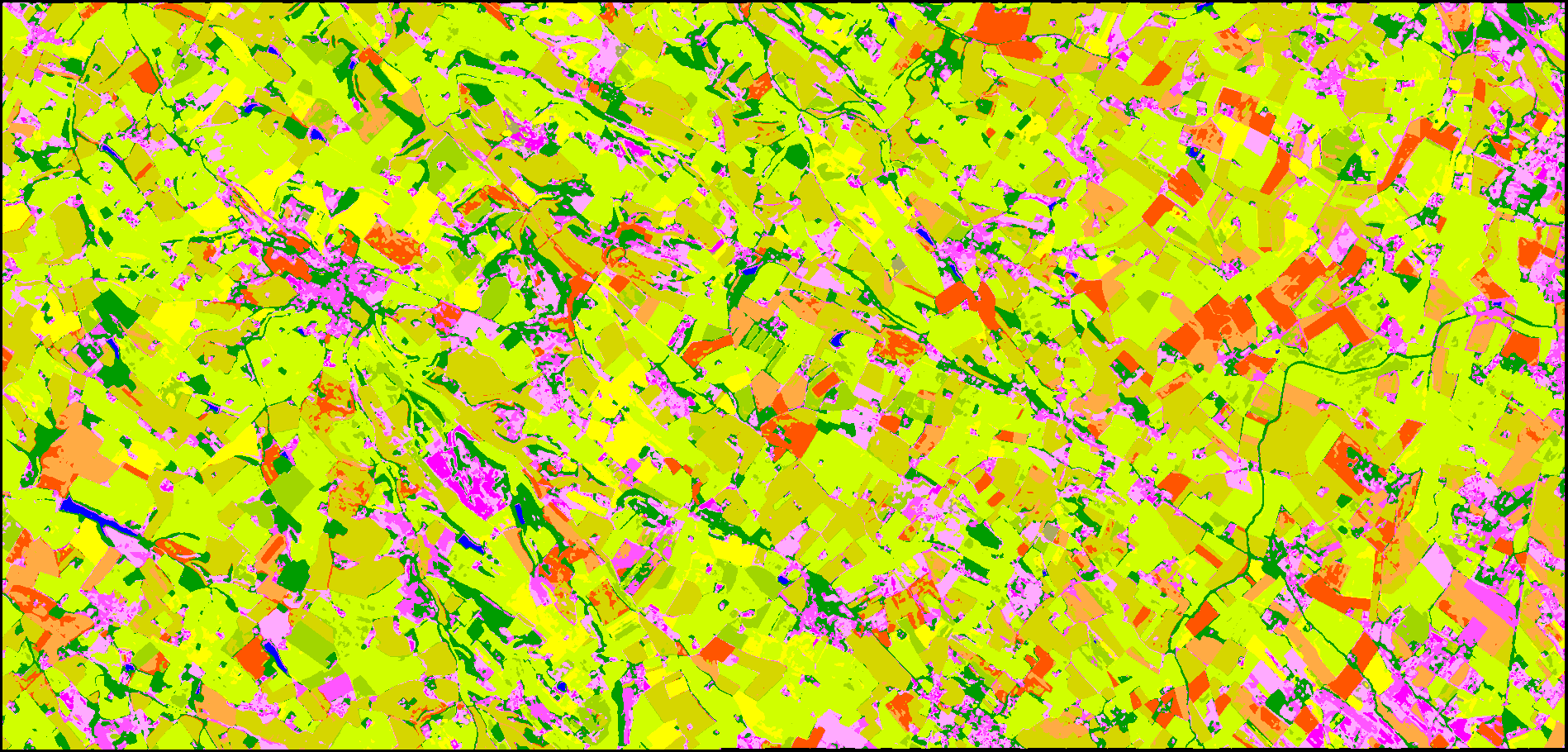
Figure 1: Classification map obtain with MLP.
Information related to the learning process are located in the model directory. For each model learned (in this labwork, we have learned only one model, but it is possible to learn several model in parallel) we have to information:
- The evolution of the training and validation losses along the interations,
- The evolution of classification metrics (OA, Kappa and class-mean F1).
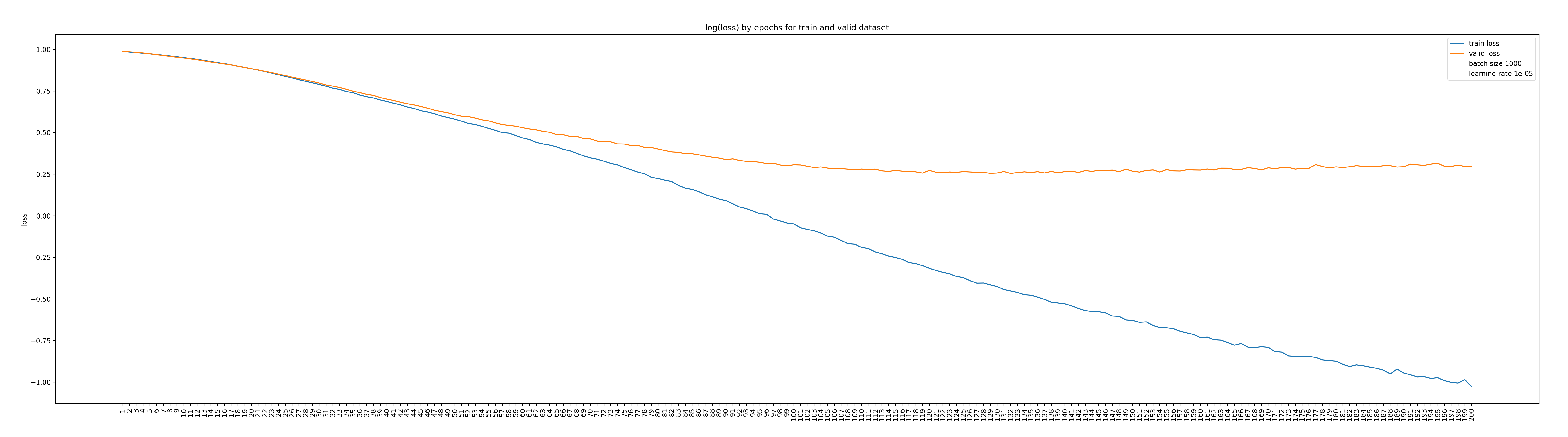
Figure 2: Training and validation losses along the iterations.
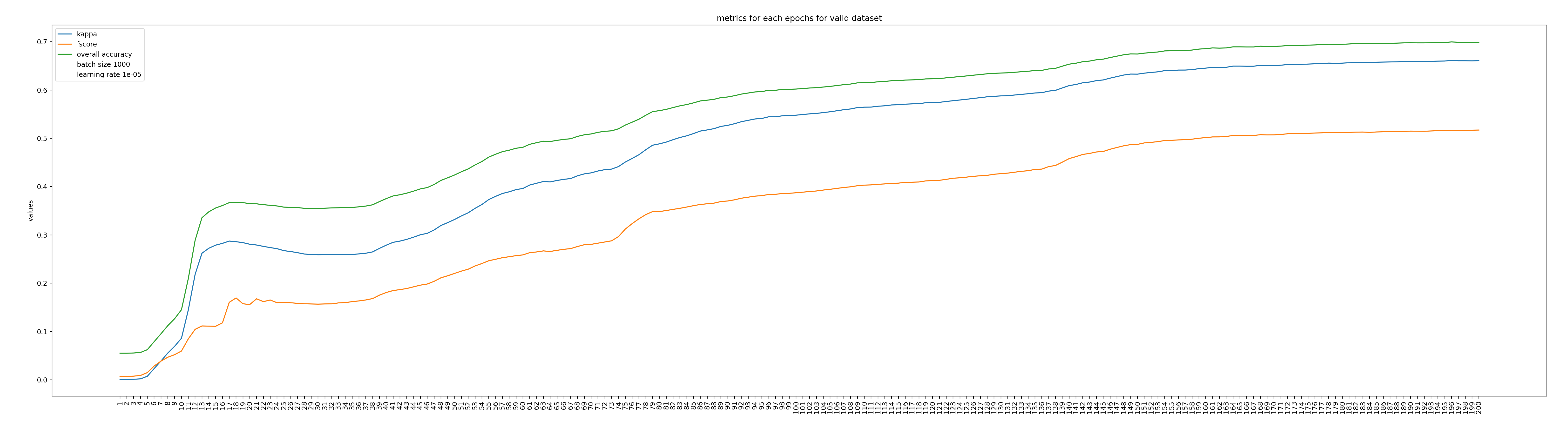
Figure 3: Classification accuracies score computed on the validation samples set along the iterations.
In Figure 2 we can see that the training loss decreased monotonously along the iteration, while the validation loss reached a plateau after a thousand of iterations. This is more or less the expected behavior when using stochastic gradient descent. Nothing wrong here. In Figure 3, we can observed that all the classification metrics increases (not monotonously!) and seems to reach a plateau at the end of the 200 epochs.
Maybe we could obtain better results by changing the parameters process: however, for this data data set, we have a limited training set as reported in the file class_statistics_seed0_learn.csv in the learningSamples directory, see Table 1.
| Class | Label | Region 1 | Total | |
|---|---|---|---|---|
| 1 | batis denses | 1 | 0 | 0 |
| 2 | batis diffus | 2 | 2000 | 2000 |
| 3 | zones ind et com | 3 | 2000 | 2000 |
| 4 | surfaces routes | 4 | 0 | 0 |
| 5 | colza | 5 | 2000 | 2000 |
| 6 | cereales à pailles | 6 | 2000 | 2000 |
| 7 | protéagineux | 7 | 2000 | 2000 |
| 8 | soja | 8 | 2000 | 2000 |
| 9 | tournesol | 9 | 2000 | 2000 |
| 10 | maïs | 10 | 2000 | 2000 |
| 11 | riz | 11 | 0 | 0 |
| 12 | tubercules/racines | 12 | 2000 | 2000 |
| 13 | prairies | 13 | 2000 | 2000 |
| 14 | vergers | 14 | 2000 | 2000 |
| 15 | vignes | 15 | 0 | 0 |
| 16 | forets de feuillus | 16 | 2000 | 2000 |
| 17 | forets de coniferes | 17 | 0 | 0 |
| 18 | pelouses | 18 | 0 | 0 |
| 19 | landes ligneuses | 19 | 2000 | 2000 |
| 20 | surfaces minérales | 20 | 0 | 0 |
| 21 | plages et dunes | 21 | 0 | 0 |
| 22 | glaciers ou neiges | 22 | 0 | 0 |
| 23 | eau | 23 | 2000 | 2000 |
| 255 | autres | 255 | 0 | 0 |
| Total | 28000 | 28000 |
You could compare the various DL models offer by iota\(^2\) in terms of classification accuracy, using multiple runs, on this data set. This requires some times and could be performed at home later!
3.2. Object based analysis
It is also possible to perform object-oriented (OBIA) classifications with Iota\(^2\). As a reminder, the “object” approach consists in classifying groups of neighbouring pixels called “object” or “segment”. It is therefore necessary to create these objects before the classification by performing a segmentation (grouping of contiguous pixels into objects). The spectral characteristics of these objects correspond to the mean and standard deviation of the spectral values of the pixels contained in the object for each band and date in the time series. Finally, a class of the nomenclature is assigned to all the pixels of the same object during the classification phase. In the literature there are several segmentation methods, however the only segmentation implemented in Iota\(^2\) is the SLIC segmentation (Simple Linear Iterative Clustering). It consists of grouping contiguous pixels by combining spectral proximity and spatial proximity to obtain a high degree of object compactness with similar sizes.
3.2.1. Object based analysis
In order to produce OBIA classification, you need to set only one parameter to choose the good builder:
builders:
{
    builders_class_name: ["i2_obia"]
}

obia:
{
    stats_used: ['mean', 'std']
}
You can also provide an file as segmentation input thanks to obia_segmentation_path parameter which can be raster or vector file. Another interesting parameter is stats_used which lists the stats you want to compute to summarize spectral value at the object scale (mean, count, min, max, std). Requesting too many stats on a long time serie can cause an error in the execution.
obia:
{
    obia_segmentation_path: "/XXX/segmentation.shp"
    stats_used: ['mean', 'std']
}
3.2.2. Contextual classification
Contextual classifications are characterized by their ability of learning the local description of the classes around the pixel of interest. The contextual features of a pixel are calculated from the proportions of each class contained in the objects (Super Pixel) to which the pixel belongs. Objects are computed with a SLIC segmentation (no parameter to set).
You can define several iterations of classifications, one iteration corresponds to :
- “pixel” classification (only in the first iteration)
- compute proportions of each class in each object
- pixel classification based on these contextual features
The number of iterations can be defined with autocontext_iterations parameter.
arg_train:
{
...
enable_autocontext : True
autocontext_iterations : 3
...
}
3.3. Use S1 data
Iota\(^2\) can combine sentinel 1 and sentinel 2 data. The first step is to filter the S1 data and then to reproject them onto the S2 grid. Read the sentinel 1 documentation to learn how.
An example S1 configuration file (not iota\(^2\) configuration file) is provided below.
[Paths]
output = /XXX/Preprocessing_S1
s1images = /XXX/s1_data/n1
srtm = /XXX/s1_data/SRTM
geoidfile = /XXX/s1_data/egm96.grd

[Processing]
tiles = 31TCJ,31TDJ
tilesshapefile = /XXX/s1_data/Features.shp
referencesfolder = /XXX/s2_data/urban
srtmshapefile = /XXX/s1_data/srtm.shp
rasterpattern = STACK.tif
gapFilling_interpolation = spline
temporalresolution = 10
borderthreshold = 1e-3
ramperprocess = 5000

[Filtering]
window_radius = 2
where the XXX is to change to your own paths.
Change your iota\(^2\) classification configuration file to include sentinel 1 data and perform the whole classification process:
- Prepare the S1 data,
- Run the classification by concatenating S1 and S2 features.
Use sentinel 1 data in a feature map builder to print the values to a feature map. See part 5 for this.
4. Use precomputed features
iota\(^2\) is originally designed to classify or analyse satellite images. In many cases, it may be useful to add additional raster data, , such as topographic variables, climate variables …, to improve the classification accuracy. Currently, it is necessary to prepare the data before the launch of iota\(^2\). This preprocessing corresponds to the reprojection and resampling of the original data so that these data are spatially “aligned” with the satellite images used for the classification. Fortunately, iota\(^2\) installs natively the OTB applications in your conda environment. The OTB application to use here is otbcli_Superimpose (https://www.orfeo-toolbox.org/CookBook/Applications/app_Superimpose.html).
Use the DEM DEM_41_5M.tif or/and DEM_45_5M.tif and Sentinel-2 images to :
- use
otbcli_Superimposeto align spatially DEM rasters with Sentinel-2 images - compute the slope and the aspect of the area thanks to
gdaldembinary (https://gdal.org/programs/gdaldem.html) (use “mnt”, “pente” and “aspect” characters in the file names) - add these new features to the configuration file as shown hereafter.
Once the reprojection has been carried out, it is sufficient to place the external data in the location indicated in the configuration file and in the corresponding tile folder (one precomputed feature by tile).
chain:
{
    ...
    list_tile: "T31TDN T31TCN"
    user_feat_path: "/path/to/precomputed/features"
    ...
}
...
userFeat:
{
    arbo:"/*"
    patterns:"mnt pente aspect"
}
user_feat_pathparameter in the “chain” section corresponds to the path where you stored texture featuresarboparameter in the new “userFeat” section corresponds to the level in the file tree (usually “/*”)patternsparameter in the new “userFeat” section given some part of the name of file(s) containing texture features
5. External Features
Iota\(^2\) provides a way to easily plug custom python code into any workflow through an interface called external features. In this labwork you will learn how to leverage iota\(^2\) large scale capabilities to parallelize custom indices computation.
5.1. Make Feature Map
Custom features can be used either in the classification workflow or be outputed as maps. We will investigate the later in this labwork. To do this, we will tell iota\(^2\) to output feature map by using the features map builder:
# add this to your config file will change the workflow of iota2
builders:
{
  builders_class_name: ["i2_features_map"]
}
As a first step, we can use existing spectral indices like the Soil Composition Index (located in external_code.py as we will see later) by appending this section to the configuration file:
external_features:
{
  functions: "get_soi"
}
# this section tells iota2 how to split data
# for parallelization and memory usage purpose
# we will cover this later
python_data_managing:
{
  chunk_size_mode: "split_number"
  number_of_chunks: 4
}
If you run iota\(^2\) multiple times by changing only the functions called by the external features, you might want to skip the preprocessing steps and only run the “writing” group:
chain :
{
  # [...]
  first_step: "writing"
  last_step: "writing"
}
- Search in the features map documentation how to modify the configuration file to prevent
iota\(^2\) from writing all the spectral bands to the feature map. - Use one of the
get_ndvi,get_ndsiorget_cariexisting functions to write another map without running all the chain.
Notice the
number_of_chunksparameter in the configuration file. It corresponds to the number of chunks each tile is split: it should be carefully set so that each task fit in memory. Each chunks can be processed in parallel using the nb_parallel_tasks command line argument. The execution graph with these parameter look like: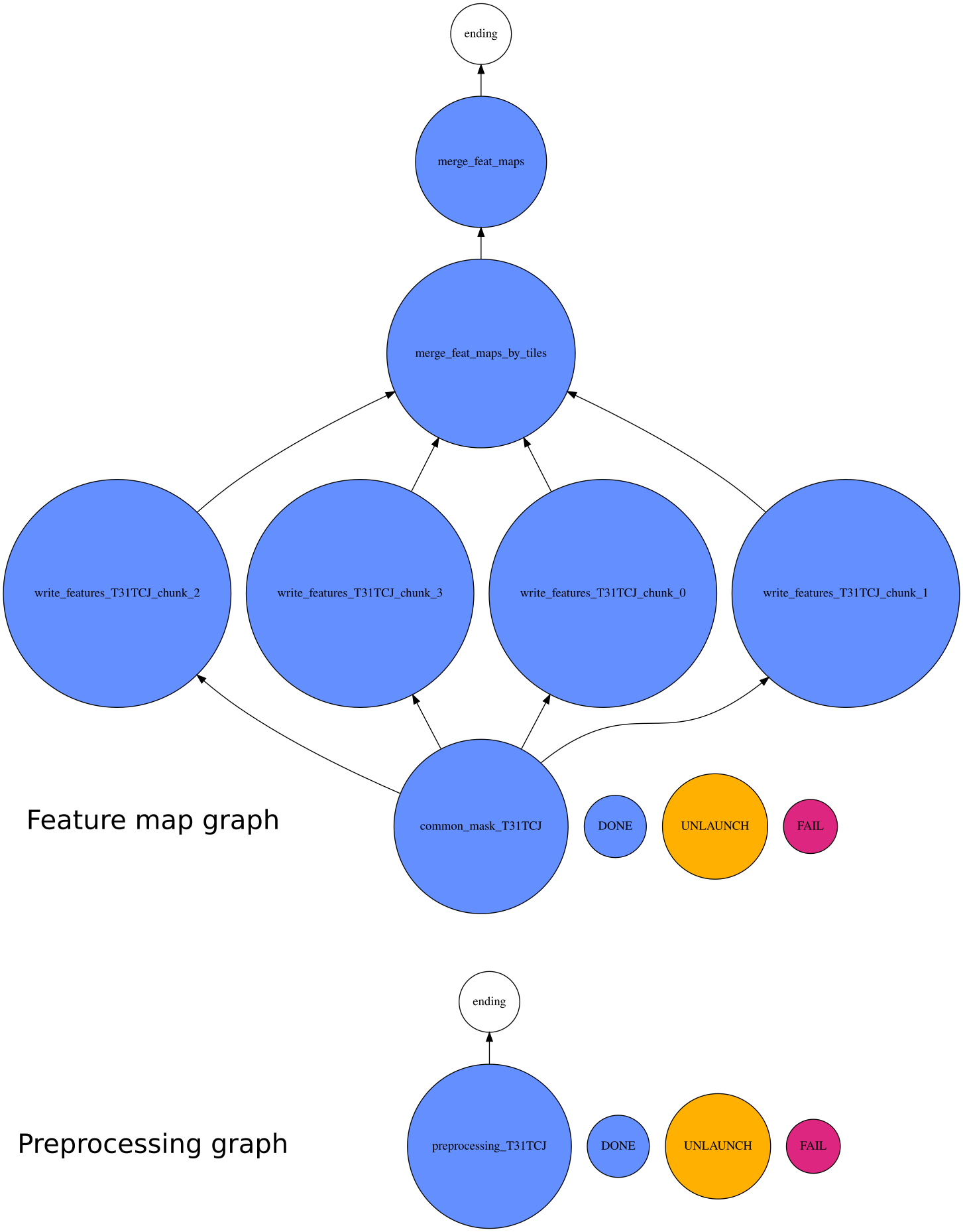
- The chunks being written can bee found in the
customFfolder before computation ends.
5.2. Create spectral indices
It’s time to write your own spectral indices. When not given the external_features / module parameter (doc), iota\(^2\) searches code in its external_code.py file. Take a look at this file to see how the data are retrieved and what is returned.
Create your own custom_code.py file with an index using multiple spectral bands and modify the configuration file to make a map of your custom index. Search in the documentation how to tell iota\(^2\) where your file is located.
You can combine multiple custom indices and add keyword arguments to your functions as shown in the documentation example. Create an index averaging bands 2,3,4,8 with weights given as function keyword arguments in the config file.
5.3. Apply spatial filters
In the previous custom indices, the output value was only using input data from the same pixel. We can write features using neighbor pixels data like this:
# add this code to your `custom_code.py` file and
# include `laplace_ndvi` to the external_features/functions section of your config file

from scipy.ndimage import laplace
import numpy as np

def laplace_ndvi(self):
    """laplacian filter over date-averaged ndvi"""
    # gets ndvi of the chunk for all dates (x,y,t)
    ndvi = self.get_interpolated_Sentinel2_NDVI()
    # average over dates
    mean_ndvi = np.mean(ndvi, axis=2)
    # apply laplace filter
    filtered = laplace(mean_ndvi, mode="constant")
    return (filtered, ["laplace_ndvi"])
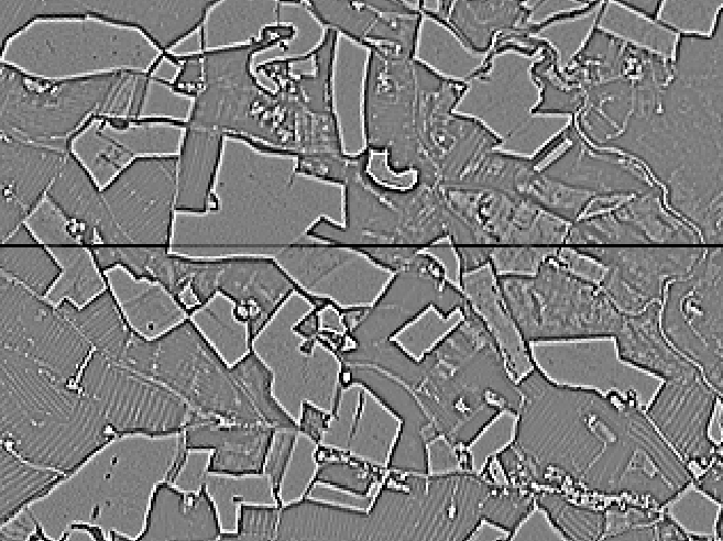
Figure 4: Screenshot of laplacian filter over mean ndvi showing border effect between chunks (dark line).
- Modify your configuration file to produce a feature map using this filter and inspect the result: You should see artifacts to due border effects, as in the figure 4. Hopefully,
iota\(^2\) provides padding options to handle such situations! - Add padding around chunks to remove these border effects. See options in https://docs.iota2.net/develop/external_features.html#how-to-use-it.
5.4. Use custom index in a classification workflow
You have learned to compute (and write on drive) your custom spectral indices and to apply spatial filtering on a feature map (or raw bands), you are now ready to perform classification using it alone, or as an additional feature.
Use the classification builder (default) with your custom index.
6. Use IOTA2 API
It is important to note that the installation of iota² provides a large number of python modules that can be used in a programming context. If iota\(^2\) does not suit some of your needs, you can access these libraries to develop your own code.
We will now consider two exercises to illustrate this ability. The first one involves OTB applications via python binding using the otb_app_bank module. The second uses the zonal_stats module to calculate the zonal statistics of a classification.
6.1. Use OTB applications with python
You can use several OTB applications via the module otb_app_bank, designed as a interface with OTB python bindings. OTB parameters (same flag names are used) are defined in a dict object which is passed to OTB functions designed in iota2/common/otb_app_bank.py. An OTB application instance is then created. You can execute it with 2 different modes by writing the output (ExecuteAndWriteOutput()) or by storing it in memory (Execute()) to use it later in another OTB application.
from iota2.common import otb_app_bank as otb

band_math = otb.CreateBandMathApplication({
    "il": [raster_path],
    "exp": "im1b1 + %s" %(constant)
})
band_math.Execute()

roi = otb.CreateExtractROIApplication({
    "in": band_math,
    "out": out_roi,
    "mode": "fit",
    "mode.fit.vect": shape_file
})
roi.ExecuteAndWriteOutput()
Considering the module otb_app_bank, complete the following script which launch a BandMath application and a ExtractROI application. It add a constant value to a raster (as example a spectral band of your choice) and clip the resulting raster with a vector file (extraction mode to -mode fit).
Note that you can either write the intermediate raster (BandMath application raster output) or use it in memory depending on the execution mode you choose (Execute() or ExecuteAndWriteOutput()).
6.2. Zonal statistics use case
After computing classification, it is often useful to calculate statistical summaries at the scale of polygons of interest (agricultural parcels, vegetation facies, municipalities, etc.). These are called zonal statistics. There is an OTB application for making zonal statistics otbcli_ZonalStatistics. It has been however implemented to calculate simple descriptive statistics (mean, std, min and max) but does not allow the computation of proportions of pixel values (corresponding for example to land use classes).
The python module zonal_stats.py supports this kind of statistic computation.
Explore the definition of the function compute_zonal_stats and try to calculate the zonal statistics of one of the classifications, you generated during the course, based on RPG zones (rpg_2018.shp) provided in course materials.
from iota2.simplification import zonal_stats as zs

list_rasters = ["classif.tif"]
zones = "rpg_2018.shp"
params = ["1:rate"]
out = "stats_classif.shp"

zs.compute_zonal_stats(tmppath, list_rasters, zones, params, out)
You can also used this functionality via bash using binary zonal_stats.py.
6.3. Use iota\(^2\) pipeline to automatize NDVI feature extraction
As seen in section 6.1, the iota\(^2\) API offers the possibility to define several applications and to chain them in a convenient way. In this section, we will show how to define custom processing using this kind of pipeline. For this labworks, we are going to extract resampled time series from pixels randomly selected in the ground truth vector file.
First, let read the configuration file, as for a regular iota\(^2\) run but in a python process (change <<path_cfg>> to the absolute path of your configuration file):
import os

from iota2.sensors.Sentinel_2 import sentinel_2
from iota2.configuration_files import read_config_file as rcf
from iota2.common.otb_app_bank import CreateExtractROIApplication

configuration_file = <<path_cfg>>
config_i2_object = rcf.read_config_file(configuration_file)
Now, we can read some information about the data to be processed (to save processing time, we only process one tile here, as indicated with the variable first_tile, but
tiles_to_compute = config_i2_object.getParam("chain", "list_tile")
i2_parameters = rcf.iota2_parameters(configuration_file)
first_tile = tiles_to_compute.split(" ")[0]

i2_sensors_parameters = i2_parameters.get_sensors_parameters(first_tile)
available_sensors_keys = list(i2_sensors_parameters.keys())
s2_instance = sentinel_2(**i2_sensors_parameters[available_sensors_keys[0]])
In this case, i2_sensors_parameters contains a dictionary with all the sensors parameters defined in the configuration file. In this labworks, we only have only Sentinel-2 data:
print(i2_sensors_parameters.keys())
Once the data variables have been read, we are ready to lazily load the full stack of feature: in our case, the Sentinel 2 gap-filled spectral data. “Lazily” means that the data cube will not fully load into the computer RAM but it will be ready to be passed as a parameter to another application, in a pipelined way.
(full_feat_stack, _), features_names = s2_instance.get_features(ram=1024)
full_feat_stack.Execute()
Roughly speaking, full_feat_stack is now a virtual stack of all the re-sampled temporal acquisition for the considered tile. We can print the name of the variables (just to fill-out our terminal!):
print(f"feature's name are : {features_names}")
So far, we have our satellite data cube ready to be processed. We now have to set up the pipeline to extract samples (it follow the sample extraction from OTB). First, define the input vector file and the output sqlite file. In the following, you can see how to read parameters value from the configuration file with the getParam method:
database = config_i2_object.getParam("chain", "ground_truth")
labels_field = config_i2_object.getParam("chain", "data_field")

statistics_file = os.path.join(
    config_i2_object.getParam("chain", "output_path"), "stats.xml"
)

samples_selection_file = os.path.join(
    config_i2_object.getParam("chain", "output_path"), "samples_selection.sqlite"
)

db_with_features_file = os.path.join(
    config_i2_object.getParam("chain", "output_path"), "samples_with_features.sqlite"
)
Next part of the code is simply the feature extraction pipeline from OTB using iota2 facility (we only extract 10 pixels per class):
from iota2.common.otb_app_bank import (
    CreateSampleSelectionApplication,
    CreatePolygonClassStatisticsApplication,
    CreateSampleExtractionApplication
)

# some statistics are needed to perfom sampling strategy
stats_app = CreatePolygonClassStatisticsApplication(
    {
        "in": full_feat_stack,
        "vec": database,
        "out": statistics_file,
        "field": labels_field,
    }
)
stats_app.ExecuteAndWriteOutput()

sampling_app = CreateSampleSelectionApplication(
    {
        "in": full_feat_stack,
        "out": samples_selection_file,
        "vec": database,
        "instats": statistics_file,
        "strategy": "constant",
        "strategy.constant.nb" : 10,
        "field": labels_field,
    }
)
sampling_app.ExecuteAndWriteOutput()

features_extraction_app = CreateSampleExtractionApplication(
    {
        "in": full_feat_stack,
        "vec": samples_selection_file,
        "field": labels_field,
        "out": db_with_features_file,
        "outfield": "list",
        "outfield.list.names": features_names,
        "ram": 4096,
    }
)

# the next line could be quite long
features_extraction_app.ExecuteAndWriteOutput()
Et voilà! You should find in the output path a sqlite file containing 10 pixels for each class, with all the spectro-temporal feature re-sampled. You can do your “expert” eyes analysis on the profile.
In this labwork, we are going to plot the NDVI for the extracted pixels:
import sqlite3
import pandas as pd
import geopandas as gpd
import matplotlib.pyplot as plt


# Load the sqlite into a geodataframe
conn = sqlite3.connect(<<path_to_db>>)
gdf = gpd.read_postgis("SELECT * from output", conn, geom_col="GEOMETRY")

# We get the NDVI features
ndvi_columns = [col_ for col_ in gdf.columns if "ndvi" in col_]
dates = [
    pd.to_datetime(date_.split("_")[2], infer_datetime_format=True)
    for date_ in ndvi_columns
]

# Here we hardcoded the class to label converter: it is extracted from nomenclature.txt
label_converter = {
    1: "batis denses",
    2: "batis diffus",
    3: "zones ind et com",
    4: "surfaces routes",
    5: "colza",
    6: "cereales à pailles",
    7: "protéagineux",
    8: "soja",
    9: "tournesol",
    10: "maïs",
    11: "riz",
    12: "tubercules/racines",
    13: "prairies",
    14: "vergers",
    15: "vignes",
    16: "forêts de feuillus",
    17: "forêts de coniferes",
    18: "pelouses",
    19: "landes ligneuses",
    20: "surfaces minérales",
    21: "plages et dunes",
    22: "glaciers ou neiges",
    23: "eau",
    24: "autres",
}

# Get the profile for pixels of each class
for label in label_converter.keys():
    # Get pixels for the considered class
    gdf_ = gdf[gdf["code"] == label][ndvi_columns]
    # Not all the define class are present in this toy exemple
    # We do not plot empty value
    if gdf_.size > 0:
        fig, ax = plt.subplots(figsize=(10, 5))
        # Within iota2 feature are stored in int16 to save memory space
        # Before casting, the pixel value is multiply by 10000 for the spectral bands
        # and by 1000 for the spectral indice.
        ax.plot(dates, gdf_.values.T/1000)
        ax.set_title(f"Class {label_converter[label]}")
        ax.set_ylim([-0.5, 1])

plt.show()
You can do many more with this, but obviously it is not related to iota\(^2\) and this is your job !

Figure 5: Spectro-temporal profile for the class sunflower.