iota2 vectorization

This chapter presents the main usage of vectorization in iota2. The process of vectorization corresponds to the conversion of a raster file (e.g. iota2 classification) into vector-based file (e.g. shapefile). Different steps are included in vectorization builder :

1. raster regularization

2. vectorization

3. generalization (simplification and smoothing)

Introduction to data

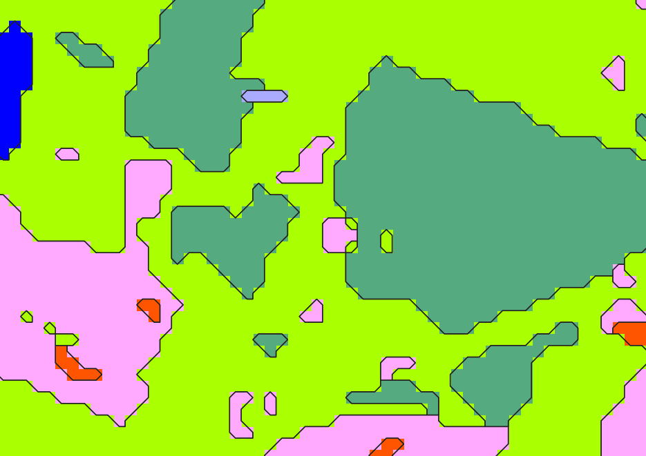
In order to find out more about how the vectorization chain works, we will use the classification raster of iota2 classification tutorial (classification tutorial). The Classif_Seed_0.tif should look like this one:

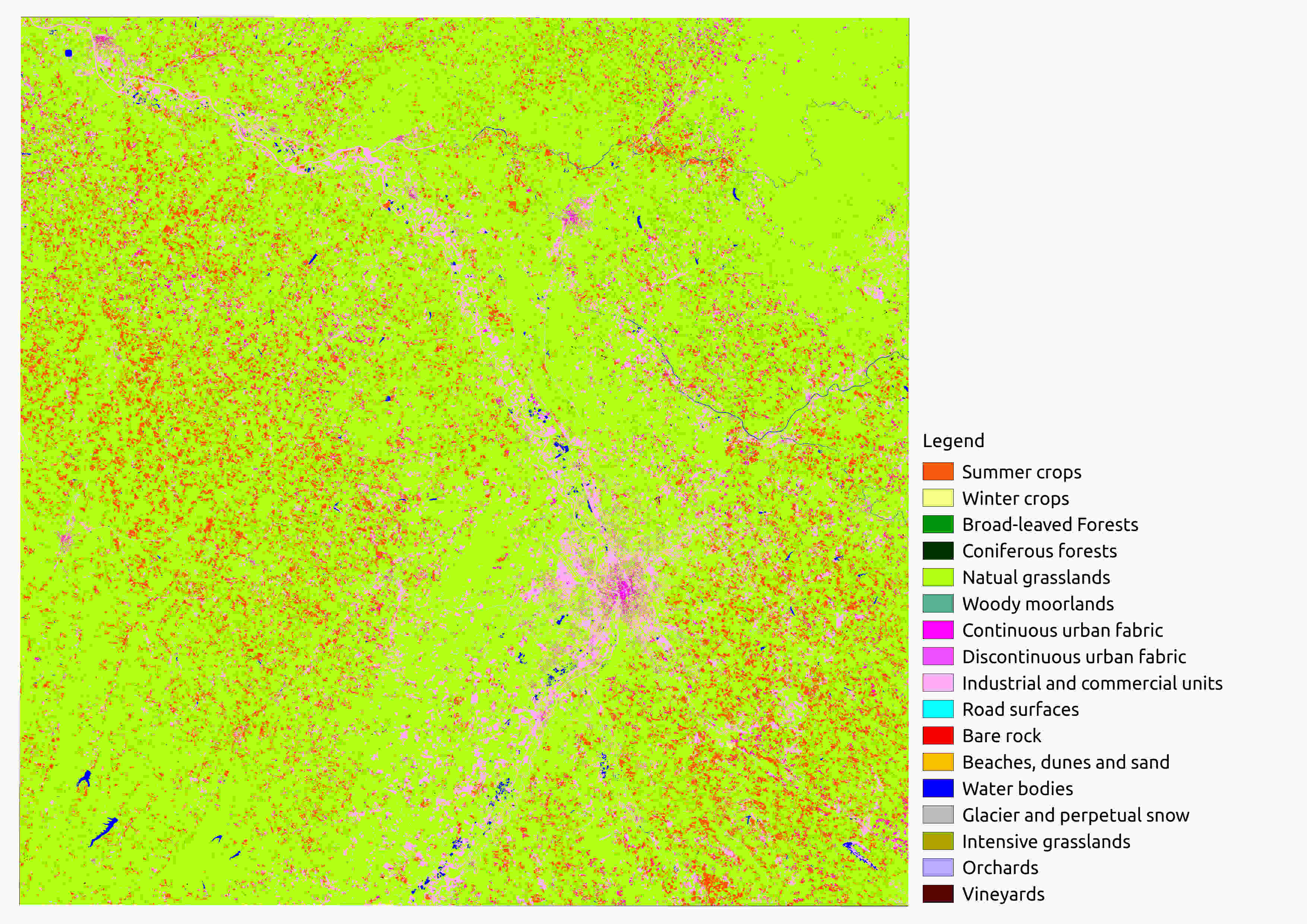
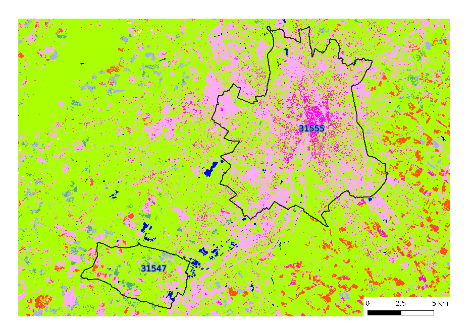
We also use a vector file of two cities in South of France, Toulouse (city code: 31555) and Seysses (city code: 31547) available in the data archive of classification tutorial.

Steps of vectorization chain

Depending on the configuration file, the vectorization chain is composed from 1 to 8 steps :

1. multi-regularization

2. raster clumping (large areas only)

3. adjacency crown raster (large areas only)

4. vectorization

5. vector-based simplification

6. vector-based smoothing

7. multi-zones extraction

8. land-cover and classifier statistics

The present tutorial focuses on the vectorization of a small geographical area. The vectorization builder was initially dedicated to large areas vectorization. For a quite small area (depending on computing resources), many parameters are useless. Conversely, the OSO-like production on large areas requires more parametrization. For large areas vectorization, you should use the gridsize parameter in order to split the treatment in tiles and perform the calculations in parallel. gridsize parameter split the treatment in gridsize x gridsize tiles.

All the parameters defined below are included in the simplification section of the configuration file.

Regularization

Principle

The python script gdal_sieve is used to “remove small raster polygons smaller than a provided threshold size (in pixels) and replaces them with the pixel value of the largest neighbour polygon”. This threshold size can be parametrized with umc1 parameter in iota2 configuration file.

An adaptive regularization is also available. Such 1 regularization removes raster polygons of specific classes and leaves those of the other classes unchanged. This adaptive regularization can be activated via a nomenclature file such as nomenclature.cfg (available in data archive). Different nested levels can be expressed :

Classes:
        {
        Level1:
        {
                Urbain:
                {
                code:100
                alias:"Urbain"
                color:"#b106b1"
                }
                ...
        }
        Level2:
        {
                Urbain dense:
                {
                code:1
                alias:"UrbainDens"
                color:"#ff00ff"
                parent:100 -> reference to Level1 codes
                }
                ...
        }
}

The lower level (e.g. level 2) corresponds to the nomenclature of the raster-based classification. Level 1 is used to group together the classes of Level2. With adaptive regularization, level 2 classes belonging to 2 different level 1 classes are not regularized.

The OSO-like regularization implies successive regularizations (normal and adaptive). If you plan to use this type of regularization process, you must enter a second threshold size parameter called umc2.

if no regularization and re-sampling are planned, leave the umc1 and rssize parameters blank.

Input parameters

simplification :
{
  umc1 : 10
  umc2 : 3
  nomenclature : '/XXXX/nomenclature_vecto.cfg'
  classification : '/XXXX/output_path_classif/final/Classif_Seed_0.tif'
  confidence : '/XXXX/output_path_classif/final/Confidence_Seed_0.tif'
  validity : '/XXXX/output_path_classif/final/PixelsValidity.tif'
  rssize : 20
  clipfile:"/XXXX/cities.shp"
  clipfield : "INSEE_COM"
  angle : True
  douglas : 10
  chunk : 10
  statslist : {"1": "rate", "2": "statsmaj", "3": "statsmaj"}
  prod:"oso"
}

classification : Classif_Seed_0.tif which is the classification raster of iota2 classification tutorial

confidence : Confidence_Seed_0.tif which is the confidence raster of iota2 classification tutorial

validity : PixelsValidity.tif which is the PixelsValidity raster of iota2 classification tutorial

umc1 : gdal_sieve searches and deletes islands of 10 pixels

rssize : spatial resolution of the output regularized raster, here 20 meters.

Vectorization

Principle

This is the core part of the vectorization process. We use Grass software libraries to manage these operations. The main reason for using this library is related to the vector format managed by Grass, i.e. the topological model. The topological model considers a vector layer as a graph of connected arcs and not as independent entities. This graph lists all the neighbourhood and membership relationships of each geographical element (node, arc, polygon) of the layer. In this context, any deformation of a vector layer based on this model does not modify the neighbourhood relations. In other words, by removing nodes from a polygon to simplify it, no holes are generated between polygons, unlike a spaghetti model.

Input parameters

  douglas : 10

angle : to smooth the corners (from the pixel geometry) of the vector layer polygons.

Vector-based simplification

Principle

In order to simplify geometries of vector layer, we provide an interface with Douglas-Peucker algorithm developed in Grass software.

Illustration of the Douglas-Peucker method

Input parameters

  chunk : 10

douglas : Douglas-Peucker tolerance for vector-based generalization

Vector-based smoothing

Principle

In order to smooth geometries of vector layer, we provide an interface with Hermite algorithm developed in Grass software.

Input parameters

hermite : Hermite Interpolation threshold for vector-based smoothing

(Multi-) Zone extraction

Principle

User can also clip the vector file, resulting from vectorization, simplification and smoothing processes, with an other vector file which can contains one (only one feature or the clipvalue parameter given) or several clipping zones. In this step, small polygons with an area smaller than the parameter “mmu” can be deleted and merged with the neighbour that shares the longest border.

Input parameters

  clipfield : "INSEE_COM"
  angle : True

mmu: Minimal Mapping Unit of output vector-based classification (projection unit)

clipfile: vector-based file to clip output vector-based classification. Vector-based file can contain more than one feature (geographical/administrative areas). An output vector-based classification is produced for each feature if no clipvalue is given (None).

clipfield: field to identify distinct geographical/administrative areas

clipvalue : here to None, to produce an output vector by distinct clipfile geometry.

Land-cover and classifier statistics

Principle

The last step of vectorization is the computing of descriptive and landcover statistics at the polygon scale. The user can request specific statistics computed on the 3 rasters produced by classification builder (Classification, Validity and Confidence rasters). As default, requested statistics are the same as the OSO-like production (parameter statslist), i.e.

  prod:"oso"

which means :

• "1": "rate": rates of classification classes (based on the output classification raster of classification builder) are computed for each polygon

• "2": "statsmaj": descriptive stats of classifier confidence are computed for each polygon by using only majority class pixels

• "3": "statsmaj": descriptive stats of sensor validity are computed for each polygon by using only majority class pixels

User can also provide a nomenclature file, already described in the Regularization step. Aliases of each class is used as field name of the output vector produced by this last step.

Finally, user can request to compress output file with parameter dozip to True.

Input parameter

  prod:"oso"

  classification : '/XXXX/output_path_classif/final/Classif_Seed_0.tif'

statslist : dictionary of requested landcover statistics, here the same as OSO production

nomenclature : description of code, color and alias of each class. Alias is used for field naming

Running the chain

After the presentation of the main parameters of the vectorization builder, you can launch a simple scenario based on these parameters.

Configuration file

As iota2 classification builder, you need a configuration file to launch this builder. The configuration file of this tutorial to provide to iota2 vectorization builder is as follow :

chain :
{
  output_path : '/XXXX/output_vecto'
  first_step : 'init'
  last_step : 'lcstatistics'
  proj : 'EPSG:2154'
}
builders :
{
  builders_class_name : ['i2_vectorization']
}
task_retry_limits : 
{
    allowed_retry : 1
    maximum_ram : 120.0
    maximum_cpu : 24
}
simplification :
{
  umc1 : 10
  umc2 : 3
  nomenclature : '/XXXX/nomenclature_vecto.cfg'
  classification : '/XXXX/output_path_classif/final/Classif_Seed_0.tif'
  confidence : '/XXXX/output_path_classif/final/Confidence_Seed_0.tif'
  validity : '/XXXX/output_path_classif/final/PixelsValidity.tif'
  rssize : 20
  clipfile:"/XXXX/cities.shp"
  clipfield : "INSEE_COM"
  angle : True
  douglas : 10
  chunk : 10
  statslist : {"1": "rate", "2": "statsmaj", "3": "statsmaj"}
  prod:"oso"
}

As you can see, we can find 3 main blocks : chain, builder and simplification. The parameters presented in previous sections are listed in the block simplification. The section builder should never be modified if you want to launch vectorization. It corresponds to the builder you want to use. Concerning the section chain as explain in the page of the classification tutorial, it contains general information such as the output path, steps you want to execute and output EPSG-style projection.

vectorization builder launch

The chain is launched with the following command line.

Iota2.py -config /XXXX/inputs/config_tutorial_vectorization.cfg -scheduler_type debug

First, the chain displays the list of all steps activated by the configuration file Full processing include the following steps (checked steps will be run):

Group regularisation:
         [x] Step 1: regularisation of classification raster
         [x] Step 2: Majority regularisation of adaptive-regularized raster
         [x] Step 3: regularisation of classification raster
         [x] Step 4: Majority regularisation of adaptive-regularized raster
Group vectorisation:
         [x] Step 5: Vectorisation of classification (Serialisation strategy)
Group simplification:
         [x] Step 6: Douglas-Peucker simplification (Serialisation strategy)
Group smoothing:
         [x] Step 7: Hermite smoothing (Serialisation strategy)
Group clipvectors:
         [x] Step 8: Clip vector files for each feature of clipfile parameters
Group lcstatistics:
         [x] Step 9: Compute statistics for each polygon of the classification
         [x] Step 10: Merge statistics

Once the processing start, a large amount of information will be printed, most of them concerning the dask-scheduler.

Did it all go well?

As explained in classification tutorial (section Did it all go well?), iota2 is packed with a logging system. Each step has its has its own log folder, available in the output\_path/logs directory. The logs directory is ordered as:

├── ClipVectors
│   ├── clip_vector_31547.err
│   ├── clip_vector_31547.out
│   ├── clip_vector_31555.err
│   └── clip_vector_31555.out
├── Clump
│   ├── clump.err
│   └── clump.out
├── html
│   ├── configuration_file.html
│   ├── environment_info.html
│   ├── genindex.html
│   ├── index.html
│   ├── input_files_content.html
│   ├── objects.inv
│   ├── output_path_content.html
│   ├── search.html
│   ├── searchindex.js
│   ├── source
│   │   ├── configuration_file.rst
│   │   ├── environment_info.rst
│   │   ├── index.rst
│   │   ├── input_files_content.rst
│   │   ├── ocs_31547_chk0.out
│   │   ├── ocs_31547_chk1.out
│   │   ├── ocs_31547_chk2.out
│   │   ├── ocs_31547_chk3.out
│   │   ├── ocs_31547_chk4.out
│   │   ├── ocs_31547_chk5.out
│   │   ├── ocs_31547_chk6.out
│   │   ├── ocs_31547_chk7.out
│   │   ├── ocs_31547_chk8.out
│   │   ├── ocs_31547_chk9.out
│   │   ├── ocs_31547.out
│   │   ├── ocs_31555_chk0.out
│   │   ├── ocs_31555_chk1.out
│   │   ├── ocs_31555_chk2.out
│   │   ├── ocs_31555_chk3.out
│   │   ├── ocs_31555_chk4.out
│   │   ├── ocs_31555_chk5.out
│   │   ├── ocs_31555_chk6.out
│   │   ├── ocs_31555_chk7.out
│   │   ├── ocs_31555_chk8.out
│   │   ├── ocs_31555_chk9.out
│   │   ├── ocs_31555.out
│   │   ├── output_path_content.rst
│   │   └── tasks_status_1.rst
│   ├── _sources
│   │   ├── configuration_file.rst.txt
│   │   ├── environment_info.rst.txt
│   │   ├── index.rst.txt
│   │   ├── input_files_content.rst.txt
│   │   ├── output_path_content.rst.txt
│   │   └── tasks_status_1.rst.txt
│   ├── _static
│   │   ├── basic.css
│   │   ├── css
│   │   │   ├── badge_only.css
│   │   │   ├── fonts
│   │   │   │   ├── fontawesome-webfont.eot
│   │   │   │   ├── fontawesome-webfont.svg
│   │   │   │   ├── fontawesome-webfont.ttf
│   │   │   │   ├── fontawesome-webfont.woff
│   │   │   │   ├── fontawesome-webfont.woff2
│   │   │   │   ├── lato-bold-italic.woff
│   │   │   │   ├── lato-bold-italic.woff2
│   │   │   │   ├── lato-bold.woff
│   │   │   │   ├── lato-bold.woff2
│   │   │   │   ├── lato-normal-italic.woff
│   │   │   │   ├── lato-normal-italic.woff2
│   │   │   │   ├── lato-normal.woff
│   │   │   │   ├── lato-normal.woff2
│   │   │   │   ├── Roboto-Slab-Bold.woff
│   │   │   │   ├── Roboto-Slab-Bold.woff2
│   │   │   │   ├── Roboto-Slab-Regular.woff
│   │   │   │   └── Roboto-Slab-Regular.woff2
│   │   │   └── theme.css
│   │   ├── doctools.js
│   │   ├── documentation_options.js
│   │   ├── file.png
│   │   ├── jquery-3.5.1.js
│   │   ├── jquery.js
│   │   ├── js
│   │   │   ├── badge_only.js
│   │   │   ├── html5shiv.min.js
│   │   │   ├── html5shiv-printshiv.min.js
│   │   │   └── theme.js
│   │   ├── language_data.js
│   │   ├── minus.png
│   │   ├── plus.png
│   │   ├── pygments.css
│   │   ├── searchtools.js
│   │   ├── underscore-1.3.1.js
│   │   └── underscore.js
│   └── tasks_status_1.html
├── LargeSimplification
│   ├── large_simpl_region_0.err
│   └── large_simpl_region_0.out
├── LargeSmoothing
│   ├── large_smooth_region_0.err
│   └── large_smooth_region_0.out
├── LargeVectorization
│   ├── large_vecto.err
│   └── large_vecto.out
├── MergeRegularization
│   ├── merge_regul2.err
│   └── merge_regul2.out
├── ProdVectors
│   ├── ocs_31547.err
│   ├── ocs_31547.out
│   ├── ocs_31555.err
│   └── ocs_31555.out
├── Regularization
│   ├── regul_2_rule_0.err
│   ├── regul_2_rule_0.out
│   ├── regul_2_rule_1.err
│   ├── regul_2_rule_1.out
│   ├── regul_2_rule_2.err
│   ├── regul_2_rule_2.out
│   ├── regul_2_rule_3.err
│   ├── regul_2_rule_3.out
│   ├── regul_2_rule_4.err
│   ├── regul_2_rule_4.out
│   ├── regul_2_rule_5.err
│   ├── regul_2_rule_5.out
│   ├── regul_2_rule_6.err
│   ├── regul_2_rule_6.out
│   ├── regul_2_rule_7.err
│   ├── regul_2_rule_7.out
│   ├── regul_2_rule_8.err
│   └── regul_2_rule_8.out
├── run_informations.txt
├── tasks_status_1.svg
├── tasks_status_2.svg
└── ZonalStatistics
    ├── ocs_31547_chk0.err
    ├── ocs_31547_chk0.out
    ├── ocs_31547_chk1.err
    ├── ocs_31547_chk1.out
    ├── ocs_31547_chk2.err
    ├── ocs_31547_chk2.out
    ├── ocs_31547_chk3.err
    ├── ocs_31547_chk3.out
    ├── ocs_31547_chk4.err
    ├── ocs_31547_chk4.out
    ├── ocs_31547_chk5.err
    ├── ocs_31547_chk5.out
    ├── ocs_31547_chk6.err
    ├── ocs_31547_chk6.out
    ├── ocs_31547_chk7.err
    ├── ocs_31547_chk7.out
    ├── ocs_31547_chk8.err
    ├── ocs_31547_chk8.out
    ├── ocs_31547_chk9.err
    ├── ocs_31547_chk9.out
    ├── ocs_31555_chk0.err
    ├── ocs_31555_chk0.out
    ├── ocs_31555_chk1.err
    ├── ocs_31555_chk1.out
    ├── ocs_31555_chk2.err
    ├── ocs_31555_chk2.out
    ├── ocs_31555_chk3.err
    ├── ocs_31555_chk3.out
    ├── ocs_31555_chk4.err
    ├── ocs_31555_chk4.out
    ├── ocs_31555_chk5.err
    ├── ocs_31555_chk5.out
    ├── ocs_31555_chk6.err
    ├── ocs_31555_chk6.out
    ├── ocs_31555_chk7.err
    ├── ocs_31555_chk7.out
    ├── ocs_31555_chk8.err
    ├── ocs_31555_chk8.out
    ├── ocs_31555_chk9.err
    └── ocs_31555_chk9.out

Output tree structure

In this section, the vectorization builder outputs available after a proper run are described.

General structure

├── logs
├── simplification
│   ├── classif_regul_clump.tif
│   ├── classif_regul.tif
│   ├── clump32bits.tif
│   ├── mosaic
│   │   ├── ...
│   ├── tiles
│   │   ├── ...
│   ├── tmp
│   │   ├── ...
│   ├── vectors
└── vectors

You can find 3 main folders on output path :

• logs : which contains all log files of each above described steps.

• simplification : folder which contains all intermediate step outputs

• vectors : which contains output vector files

Regularization / Clump

Regularization step produces 3 outputs :

• classif_regul.tif : final regularization file

• clump32bits.tif : clump raster which corresponds to the segmentation of regularization raster

• classif_regul_clump.tif : the concatenation of the two former ones

Classif_Seed_0.tif vs. classif_regul.tif

You can observe an important reduction of small raster polygons.

Vectorization

Once regularization done, vectorization is launched and output vector file is stored in mosaic folder. Internal naming is used in the form of tile_'clipfield'_'clipvalue'.shp

├── simplification
│   ├── ...
│   ├── mosaic
│   │   ├── tile_INSEE_COM_0.dbf
│   │   ├── tile_INSEE_COM_0.prj
│   │   ├── tile_INSEE_COM_0.shp
│   │   └── tile_INSEE_COM_0.shx
│   │   └── ...

classif_regul.tif vs. tile_INSEE_COM_0.shp

Each raster polygon is vectorized based on a topological process.

Vectorization output in black (we can see the effect of angle parameter)

Simplification

The Douglas-Peucker simplification is done and also stored in mosaic folder with suffix _douglas.

├── simplification
│   ├── ...
│   ├── mosaic
│   │   ├── ...
│   │   ├── tile_INSEE_COM_0_douglas.dbf
│   │   ├── tile_INSEE_COM_0_douglas.prj
│   │   ├── tile_INSEE_COM_0_douglas.shp
│   │   ├── tile_INSEE_COM_0_douglas.shx
│   │   └── ...

tile_INSEE_COM_0.shp vs. tile_INSEE_COM_0_douglas.shp

Smoothing

The Hermite smoothing is done and also stored in mosaic folder with suffix _hermite.

├── simplification
│   ├── ...
│   ├── mosaic
│   │   ├── ...
│   │   ├── tile_INSEE_COM_0_douglas_hermite.dbf
│   │   ├── tile_INSEE_COM_0_douglas_hermite.prj
│   │   ├── tile_INSEE_COM_0_douglas_hermite.shp
│   │   ├── tile_INSEE_COM_0_douglas_hermite.shx
│   │   └── tile_INSEE_COM_0_douglas_hermite.shx

tile_INSEE_COM_0_douglas.shp vs. tile_INSEE_COM_0_douglas_hermite.shp

At the end of this step, operations on geometries of classification vector file are finished. You can observe the removal of small polygons with an area under the mmu size (here : 10 pixels)

Clipping

Once vector operations are done, output vector files *_douglas_hermite.shp are clipped with clip file provided in configuration file. It produces one output vector file by different values of clip field in simplification/vectors folder. Naming strategy is as followed 'prefix'_'value'.shp (value : value(s) of clip field).

├── simplification
│   ├── ...
│   └── vectors
│       ├── ocs_31547.dbf
│       ├── ocs_31547.prj
│       ├── ocs_31547.shp
│       ├── ocs_31547.shx
│       ├── ocs_31555.dbf
│       ├── ocs_31555.prj
│       ├── ocs_31555.shp
│       └── ocs_31555.shx

Example of clipping (clip_field = “INSEE_COM” & clip_value = 31547)

Zonal Statistics

The final step compute landcover (rate of classes), classifier (confidence mean) and sensor (validity) statistics on classification output rasters (classification builder) for each output vector features. Final output vectors are stored in vectors folder at the root of output path.

├── simplification
│   ├── ...
└── vectors
    ├── ocs31547.dbf
    ├── ocs31547.prj
    ├── ocs31547.shp
    ├── ocs31547.shx
    ├── ocs31555.dbf
    ├── ocs31555.prj
    ├── ocs31555.shp
    ├── ocs31555.shx

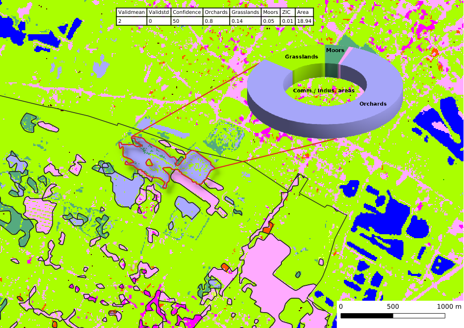
Example of rates of landcover classes for this vector feature