Region based classification fusion
The standard workflow produces an entire tile classification for each region that intersects a given tile. After that, the regions vector file is used to crop each classification before merging them into one single classification per tile without overlaps.
This procedure can create artefacts around the boundaries of the regions if the models give different classes to adjacent pixels belonging to different regions. The following figure shows the kind of issues which can occur. The region boundary clearly appears in the produced map.
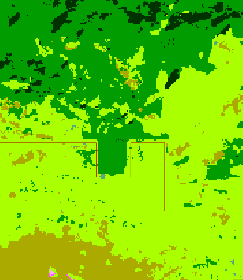
Example of boundary artefact
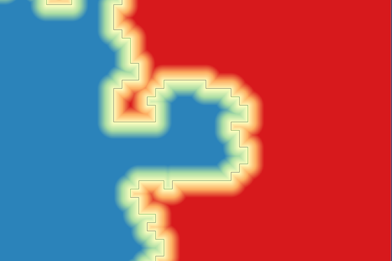
A simple solution is proposed to attenuate this kind of effect. The main idea is to compute a weighted fusion of model outputs according to the distance of a pixel with respect to the region boundary. Since the classifiers are able to provide a probability for each pixel to belong to each class, the weighted sum of probabilities is computed and the class with the highest value is chosen.
The weighted probabilities are only computed inside a buffer area around the region boundaries. Pixels outside of the buffer belong to the label predicted by the region’s model.
For a given region and its boundary with respect to one of its adjacent regions, we define the interior and the exterior boundaries. The interior boundary is the boundary of the buffer inside the considered region. The exterior boundary is the boundary of the buffer inside the adjacent region. Note that the buffer can have different sizes in the interior and the exterior sides.
The pixel’s distance to the boundary is computed using the Danielsson algorithm which computes euclidian distance in images.
The weight is computed with a linear expression, in order to provide a weight of 1 at the interior boundary, and a weight of 0 at the exterior boundary. A epsilon value is required to avoid O in weights if the region geometry is complex. This value is a float which must be storable as UINT16 once multiplied by 1000, i.e the smallest value accepted is 0.001. Under this value, the weight is set to 0. At the original boundary, the weight is set to be 0.5.
After the classification of each region by a classifier which provides per class probability, a decision is taken by weighting the probability of each model by the pixel’s weight.
How to enable the boundary fusion mode
To enable the bonudary fusion, several parameters must be set.
Most of them are grouped in the arg_classification section of the configuration file.
arg_classification :
{
    enable_probability_map: True
    generate_final_probability_map: False
    boundary_comparison_mode:False
    enable_boundary_fusion: True
    boundary_interior_buffer_size: 100
    boundary_exterior_buffer_size: 500
    boundary_fusion_epsilon: 0.001
}
It is mandatory to enable the probability map production, as it is the main input of the workflow. The classifier set in the arg_train section must provide probabilities.
It is possible to set different values for the interior and exterior boundary sizes. Note that the unit is in meters here. The buffer size is converted in pixels according to the working resolution.
Using the comparison mode
It can be useful to compare the standard workflow and the fusion approach we just described.
To this end, an option was added boundary_comparison_mode. If enabled, the final folder is slighty modified to provide both versions of all products: RESULTS.txt, Confusion matrix, land-cover and confidence maps, in two separate subfolders: standard and boundary. In the final folder, files containing conditional validation for the boundary areas are provided.
These use the following convention:
\(C_s\) the fusion after masking the classification with regions;
\(C_b\) the fusion using boundary area and probabilities.
Four matrices and their associated metrics are computed:
\(conf(C_s,Yref)\): confusion matrix between \(C_s\) and the reference samples (not used during training) on the boundary
\(conf(C_b,Yref)\): confusion matrix between \(C_b\) and the reference samples (not used during training) on the boundary
\(conf(C_s|Y=Yref, C_b)\): confusion matrix between \(C_s\) only when the prediction of \(C_s\) is correct (correct = equal to the reference samples not used during training) and \(C_b\)
\(conf(C_b|Y=Yref, C_s)\): confusion matrix between \(C_b\) only when the prediction of \(C_b\) is correct (correct = equal to the reference samples not used during training) and \(C_s\)